
Training RegNets for tf.keras.applications
Published:
This blog post is about sharing our experience of training 24 RegNet models for tf.keras.applications.
Prologue
tf.keras.applications is a set of built-in models in TensorFlow-Keras. They are pretrained on ImageNet-1k, and are just one function call away. This makes life easier for the ML folks as they have ready-to-go models at their disposal. RegNets are highly efficient and scalable models proposed by Facebook AI Research (FAIR). They are used in works like SEER which need models that can scale to billions and billions of parameters. In submitting a PR to Keras, I implement and train 24 RegNet models of varying complexity to tf.keras.applications.
Even though I was responsible for the primary development work on the PR as well as training the models, I received great help from the community which makes it truly collaborative.
I performed several experiments with these models, because the reported accuracies could not be reproduced using the hyperparameters provided in the paper. This blog post is a record of these experiments I tried and how they panned out.
Acknowledgements:
I sincerely thank the Keras team for allowing me to add these models. Huge thanks to the TPU Research Group (TRC) for providing TPUs for the entire duration of this project, without which this would not have been possible. Thanks a lot to Francois Chollet for allowing this and guiding me throughout the process. Thanks to Qianli Scott Zhu for his guidance in building Keras from source on TPU VMs. Thanks to Matt Watson for his support regarding grouped convolutions. Special thanks to Lukas Geiger for his contributions to the code. Last but not least, thanks a ton to Sayak Paul for his continuous guidance and encouragement.
The Basics
About the paper
The paper “Designing Network Design Spaces” aims to systematically deduce the best model population starting from a model space that has no constraints. The paper also aims to find a best model population, as opposed to finding a singular best model as in works like NASNet. The outcome of this experiment is a family of networks which comprises models with various computational costs. The user can choose a particular architecture based upon the need.
About the models
Every model of the RegNet family consists of four Stages. Each Stage consists of numerous Blocks. The architecture of this Block is fixed, and three major variants of this Block are available: X Block, Y Block, Z Block. Other variants can be seen in the paper, and the authors state that the model deduction method is robust and RegNets generalize well to these block types. The number of Blocks and their channel width in each Stage is determined by a simple quantization rule put forth in the paper. More on that in this blog. RegNets have been the network of choice for self supervised methods like SEER due to their remarkable scaling abilities.
The Pull Request:
Before opening a pull request which requires large amounts of work, it is advisable to consult the team first so that there is no conflict of interest. After getting a solid confirmation from the Keras team, I started working on the code. You can check out our discussion here. Below is a small snippet from our conversation:
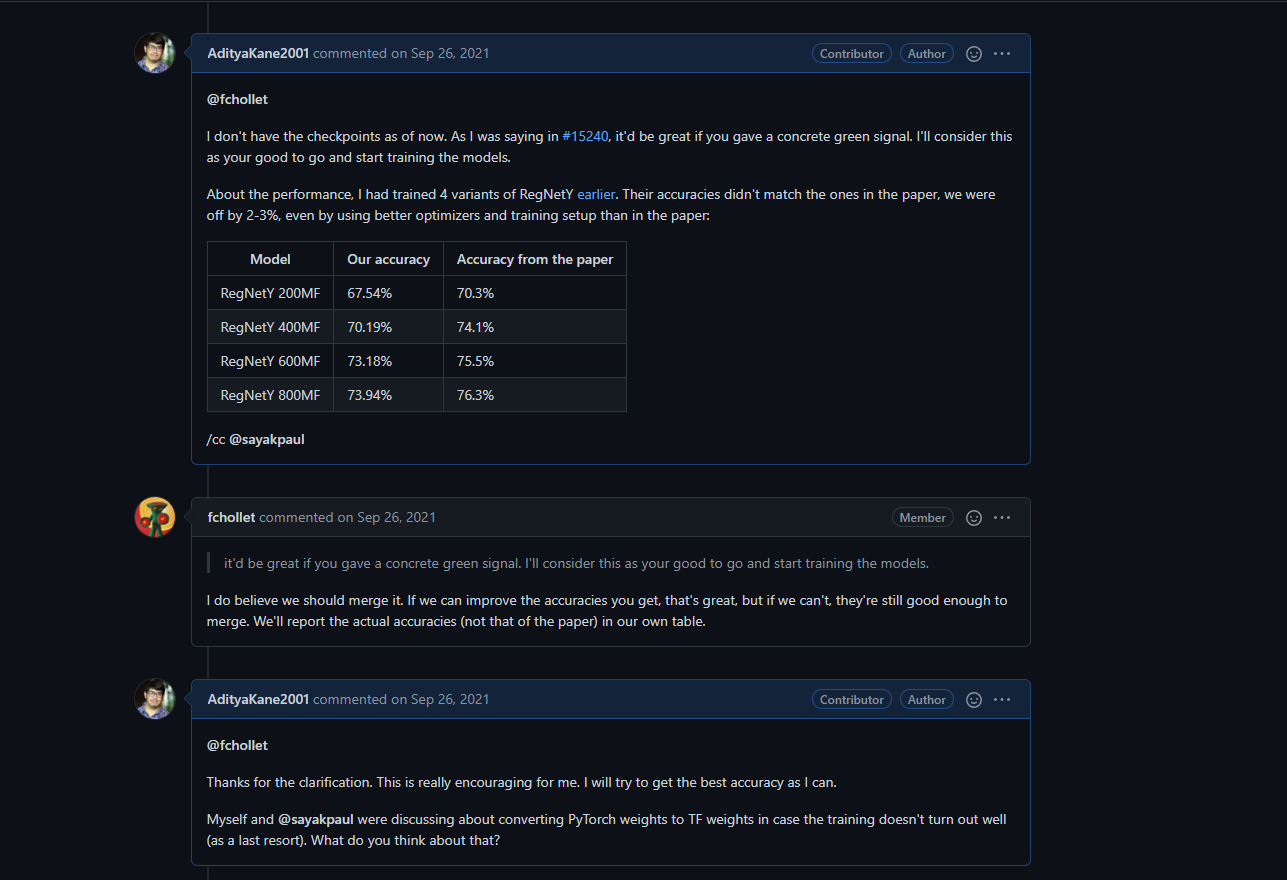
François Chollet and the Keras team were super supportive and made merging the PR a smooth process. I express my heartfelt gratitude to the team for their help. Even though I had 24 models to implement, the basic code was fairly straightforward. Thus, I was able to create a PR with the code and get reviews from the team quickly. Check out the PR here.
Training the models:
General Setup
I mainly used the TPUv3-8 Node for training. It has a 96-core VM with around 335 GB RAM, which handles heavy preprocessing with ease. After preprocessing raw images/posts/training-regnets were resized to 224x224 as mentioned in the paper. I used multiple TPU Nodes simultaneously to allow running many experiments in parallel. This reduced the experimentation time considerably.
The code used for training is available here.
In this section, I simply jot down the takeaways and methods I used for achieving this performance. Input pipeline I trained these models on the powerful TPU-v3 (thanks to TRC). This meant that I had to employ a lightning-fast input pipeline. Also, the input pipeline must be static, which means I cannot have abrupt changes in the preprocessing graph at runtime (since the preprocessing functions are optimized using AutoGraph). As per the requirements of TPUs, I stored the ImageNet-1k TFRecords on a GCS bucket and employed an interleaved dataset read.
Learning point: It is important to implement augmentations in the most efficient and stable way possible and minimize slow and redundant ops in the process.
Some chunks of the code are repeated, but this guarantees that the function remains pure. Here being pure simply means absence of break statements, which would otherwise cause the graph to change arbitrarily. One can also see, for example, the variable w_crop is cast to tf.int32exactly once in the entire function call. It is important to do such optimizations, because we are working with a single image at a time and not a batch of images/posts/training-regnets. You can check out the code here. The actual code was not included in this blog for the sake of brevity.
We can see that some chunks of the code are repeated, but this guarantees that the function remains pure. Here being pure simply means absence of break statements, which would otherwise cause the graph to change arbitrarily. One can also see, for example, the variable w_crop is cast to tf.int32 exactly once in the entire function call. It is important to do such optimizations, because we are working with a single image at a time and not a batch of images/posts/training-regnets.
Apart from inception style cropping, the implementation of the remaining input pipeline was fairly simple. I used inception cropping, channel-wise PCA jitter, horizontal flip and mixup.
PCA jitter:
    def _pca_jitter(self, image, target):
        """
        Applies PCA jitter to images/posts/training-regnets.
        Args:
            image: Batch of images/posts/training-regnets to perform random rotation on.
            target: Target tensor.
        Returns:
            Augmented example with batch of images/posts/training-regnets and targets with same dimensions.
        """

        aug_images/posts/training-regnets = tf.cast(image, tf.float32) / 255.
        alpha = tf.random.normal((self.batch_size, 3), stddev=0.1)
        alpha = tf.stack([alpha, alpha, alpha], axis=1)
        rgb = tf.math.reduce_sum(
            alpha * self.eigen_vals * self.eigen_vecs, axis=2)
        rgb = tf.expand_dims(rgb, axis=1)
        rgb = tf.expand_dims(rgb, axis=1)

        aug_images/posts/training-regnets = aug_images/posts/training-regnets + rgb
        aug_images/posts/training-regnets = aug_images/posts/training-regnets * 255.

        aug_images/posts/training-regnets = tf.cast(tf.clip_by_value(aug_images/posts/training-regnets, 0, 255), tf.uint8)

        return aug_images/posts/training-regnets, target
Mixup:
    def _mixup(self, image, label, alpha=0.2) -> Tuple:
        """
        Function to apply mixup augmentation. To be applied after
        one hot encoding and before batching.
        Args:
            entry1: Entry from first dataset. Should be one hot encoded and batched.
            entry2: Entry from second dataset. Must be one hot encoded and batched.
        Returns:
            Tuple with same structure as the entries.
        """
        image1, label1 = image, label
        image2, label2 = tf.reverse(
            image, axis=[0]), tf.reverse(label, axis=[0])

        image1 = tf.cast(image1, tf.float32)
        image2 = tf.cast(image2, tf.float32)

        alpha = [alpha]
        dist = tfd.Beta(alpha, alpha)
        l = dist.sample(1)[0][0]

        img = l * image1 + (1 - l) * image2
        lab = l * label1 + (1 - l) * label2

        img = tf.cast(tf.math.round(tf.image.resize(
            img, (self.crop_size, self.crop_size))), tf.uint8)

        return img, lab
Random horizontal flip:
    def random_flip(self, image: tf.Tensor, target: tf.Tensor) -> tuple:
        """
        Returns randomly flipped batch of images/posts/training-regnets. Only horizontal flip
        is available
        Args:
            image: Batch of images/posts/training-regnets to perform random rotation on.
            target: Target tensor.
        Returns:
            Augmented example with batch of images/posts/training-regnets and targets with same dimensions.
        """

        aug_images/posts/training-regnets = tf.image.random_flip_left_right(image)
        return aug_images/posts/training-regnets, target
– PCA jitter and random horizontal flip were suggested in the paper, whereas addition of mixup was inspired by the papers Revisited ResNets.
Effect of weight decay on training
Weight decay is a regularization technique where we penalize the weights for being too large. Weight decay is a battle-tested method and is often used when training deep neural networks. A small note, I used decoupled weight decay and not the conventional implementation of weight decay.
I saw increasing the weight decay too much made it difficult for the model to converge. However, small weight decay caused the model to have near-constant accuracy during the final epochs. These observations suggest the weight decay is a strong regularizer, especially for smaller models. Inspired by the paper “Revisiting ResNets: Improved Training and Scaling Strategies”, I kept the weight decay same for large models, since mixup was increased simultaneously.
Learning point: Weight decay is a strong regularizer. It is advisable to reduce weight decay or keep it the same for large models, where other augmentations or regularizers are being used simultaneously.
Finally, I used a constant weight decay of 5e-5 for all models, which was suggested in the original paper.
Regularization as a function of model size It is empirically known that increasing augmentation of regularization results in better performance. Conforming to this, I gradually increased the strength of mixup augmentation as the model size increased. I saw good results using this simple technique.
Learning point: Increase augmentations and regularization when increasing model size.
Smaller models are difficult to train
I had to train 12 variants of RegNetX and RegNetY each. This included small models which don’t have as many parameters as the larger ones. It is speculated that these models simply do not have enough capacity to hold the given information in them. They tend to underfit and the solution is seldom as simple as adding augmentation. The best starting point in most cases was low regularization and medium augmentation. I could tune the rest of the hyperparameters from there. These models took a lot of time to fine-tune and train, whereas the larger models had more flexibility. Smaller models are sensitive to small changes in regularization or augmentation.
Learning point: Do a hyperparameter search for small models. Repeat the search as the size of models increases.
Noteworthy learnings:
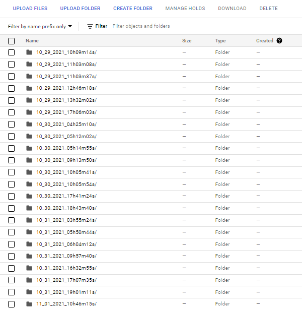
Use multiple copies of the data if possible It was observed the training would stop abruptly and would be stuck at the end of an epoch. I use the
tf.data.Dataset.interleavemethod which reads data from multiple TFRecords simultaneously. During this read operation, the TFRecords are unavailable to other processes. I used to train multiple models in parallel, and thus they constantly needed to read data from the same bucket. Thus, to counter this, I created multiple copies of the TFRecords and saved them in different buckets. This reduced collisions and the problem reduced substantially.Dump logs at a single location While training a number of models, maintaining the logs may get out of hand. The best way, in my opinion, is to dump all the raw logs at one location. In our case, I organized the logs and checkpoints of the models using the time and date of training. This made it easier to locate and use the checkpoints where needed. Following is a snap of the same:
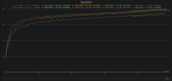
Use automation to reduce cognitive load Managing many experiments simultaneously quickly becomes a difficult task. Automating the things which you need to do repeatedly is an extremely useful thing to do from the beginning. For example, one can use Weights and Biases (W&B) to automatically track all experiments. It is useful to log the hyperparameters along with the runs in W&B rather than feeding them manually. These seemingly small things reduce a ton of cognitive load, so you can actually focus on what’s important - running experiments. Following is a snapshot of our runs:
Gain intuitions of how the model might react to certain changes to hyperparameters After working on a single architecture for days or months, you may notice patterns in the performance of models. This helps in building intuitions of how the model might react to different changes in hyperparameters. Using this newfound intuition, you might be able to come up with ideas which might help in increasing performance. For example, using a slightly higher weight decay for RegNetY004 leads to sudden increase followed by a decrease of accuracy at the end of the run, but using a lower weight decay flattens this out. This implies that usage of a more aggressive augmentation policy along with lower weight decay may help in training, in this case. In similar fashion, one can spot changes in hyperparameters which lead to significant improvements.
Finally, here are the results. In the following tables, I compare our results with the paper. The last column has the hyperparameters which are different from the original implementation.
X variant
| Model | Paper | Ours | Diff | Comments |
|---|---|---|---|---|
| X002 | 68.9 | 67.15 | 1.75 | adamw, area_factor=0.25 |
| X004 | 72.6 | 71.22 | 1.38 | adamw, area_factor=0.08 |
| X006 | 74.1 | 72.37 | 1.73 | adamw, area_factor=0.08 |
| X008 | 75.2 | 73.45 | 1.75 | adamw, area_factor=0.08 |
| X016 | 77 | 75.55 | 1.45 | adamw, area_factor=0.08, mixup=0.2 |
| X032 | 78.3 | 77.09 | 1.21 | adamw, area_factor=0.08, mixup=0.2 |
| X040 | 78.6 | 77.87 | 0.73 | adamw, area_factor=0.08, mixup=0.2 |
| X064 | 79.2 | 78.22 | 0.98 | adamw, area_factor=0.08, mixup=0.3 |
| X080 | 79.3 | 78.41 | 0.89 | adamw, area_factor=0.08, mixup=0.3 |
| X120 | 79.7 | 79.09 | 0.61 | adamw, area_factor=0.08, mixup=0.4 |
| X160 | 80 | 79.53 | 0.47 | adamw, area_factor=0.08, mixup=0.4 |
| X320 | 80.5 | 80.35 | 0.15 | adamw, area_factor=0.08, mixup=0.4 |
Y variant
| Model | Paper | Ours | Diff | Comments |
|---|---|---|---|---|
| Y002 | 70.3 | 68.51 | 1.79 | adamw, WD=1e-5, area_factor=0.16 mixup=0.2 |
| Y004 | 74.1 | 72.11 | 1.99 | adamw, WD=1e-5, area_factor=0.16, mixup=0.2 |
| Y006 | 75.5 | 73.52 | 1.98 | adamw, area_factor=0.16, mixup=0.2 |
| Y008 | 76.3 | 74.48 | 1.82 | adamw, area_factor=0.16, mixup=0.2 |
| Y016 | 77.9 | 76.95 | 0.95 | adamw, area_factor=0.08, mixup=0.2 |
| Y032 | 78.9 | 78.05 | 0.85 | adamw, area_factor=0.08, mixup=0.2 |
| Y040 | 79.4 | 78.2 | 1.2 | adamw, area_factor=0.08, mixup=0.2 |
| Y064 | 79.9 | 78.95 | 0.95 | adamw, area_factor=0.08, mixup=0.3 |
| Y080 | 79.9 | 79.11 | 0.69 | adamw, area_factor=0.08, mixup=0.3 |
| Y120 | 80.3 | 79.45 | 0.85 | adamw, area_factor=0.08, mixup=0.4 |
| Y160 | 80.4 | 79.71 | 0.69 | adamw, area_factor=0.08, mixup=0.4 |
| Y320 | 80.9 | 80.12 | 0.78 | adamw, area_factor=0.08, mixup=0.4 |
Conclusion
I trained a total of 24 models for this PR. It was an enriching experience and I hope that these models will be used by many developers. It was a great learning experience, and I hope to continue contributing to TensorFlow & Keras in the near future again.